- Research
- Open access
- Published:
FPGA implementation of JPEG encoder architectures for wireless networks
EURASIP Journal on Embedded Systems volume 2017, Article number: 10 (2017)
Abstract
Due to its relative simplicity, the JPEG compression algorithm requires less hardware or software resources with respect to new compression algorithms, for example the JPEG2000 and the JPEG XR. This makes it suitable for low-power applications. Moreover, features embedded in the JPEG2000 and the JPEG XR, such as the scalability of the image stream, can be added to the main JPEG core, making an encoder useful for example in a video surveillance wireless network. Nevertheless, actual JPEG dedicated hardware realizations do not implement many features of the compression standard. In this work, we developed several JPEG encoder architectures with full real-time reconfigurability and support for the restart intervals and, for a simple scalability mechanism, the scan scheme. These features make the architectures suitable for the use in low-bandwidth, low-power wireless networks. The JPEG encoder architectures have been developed starting from a SystemC model and then implemented in a FPGA.
1 Introduction
In today’s world, every day we get a newer, faster, and cheaper technology. This is particularly true for processing and communication devices and any kind of sensors and networks. Wireless sensor networks become every day more powerful and ubiquitous, and it is becoming possible to design a network for every purpose. Among the others, video surveillance is becoming one of the most promising applications of wireless sensor networks [1–6].
Wireless sensor networks are flexible and ready-to-use: to install a network, we simply have to deploy the sensors where we want to. But this flexibility comes with three main prices: high sensitivity to the noise in the channel, limited bandwidth, and limited power supply. In a wireless image sensor network, this means that we have to compromise among the quality of the image to be transmitted, the number of images per second that can be transmitted, and the power dissipated for image processing and transmission. To find the optimum solution for the particular application we are working with, image processing and compression algorithms, sensor node architecture, wireless protocol from application layer to physical layer, and network topology must be analyzed and all the parameters of the sensor network should be tuned with system level simulations.
In this paper, we focus on the usual solution to the bandwidth limitations: the image compression. Image compression is used to reduce the data amount to be transmitted, but usually, this reduction comes with a loss in the image quality and a greater sensitivity to channel noise. Moreover, the image compression algorithm introduces complexity and, hence, higher power consumption. From this point of view, it is important to design architectures with a good compromise between performances and complexity.
Nowadays, the JPEG is the most used image compression algorithm, mainly because of its relatively easy implementation and of its fair compromise between complexity and compressed image quality. The PSNR of a JPEG image is only a few dB lower than that of the same JPEG 2000 image, while the compression time of the former is seven times lower than the latter [7]. Moreover, the noise resilience of a JPEG image is comparable to that of a JPEG 2000 one in many cases [7], and the advanced features defined by the JPEG 2000 standard (i.e., the scalability and the Region-Of-Interest) are defined by the JPEG standard and its extensions too. While these extensions to the JPEG main core may be less efficient than those of the JPEG 2000, in many applications (especially the battery-powered ones), the low complexity of the JPEG can effectively balance this lower efficiency.
Several research have been devoted to the design of architectures for a JPEG encoder. In [8], for example, an architecture for a single-chip JPEG codec is described, in [9, 10], an architecture for VLSI implementation, and in [11, 12], another architecture for the implementation in FPGA. The architectures described in [9, 11] are similar and very efficient, and they are designed to maximize the throughput by the extensive use of the pipeline, while the architecture in [8] presents limitations due to the poor DCT implementation. Another noteworthy architecture for VLSI implementation is presented in [13], which also takes into account for the acquisition of the image to be compressed from a CMOS sensor. All these architectures have several limitations: the implementations are limited to the very basic functionality of the JPEG algorithm, which is the mode of operation known as “JPEG Baseline” [14, 15]. This choice is motivated by the fact that the JPEG Baseline is the “version” of the JPEG most widely supported by free and commercial software.
However, besides these basic functionalities, there are many features that the standard defines and anyone implemented. These features are useful and sometimes indispensable in a wireless network: in particular, but not only, the restart markers can be used to improve the image noise resilience, and the scan mechanism as a simple way to add scalability to the image stream, useful for adaptive bandwidth utilization.
Moreover, the architectures reported in [8, 9, 11, 13] have low reconfigurability: basically, they use small ROMs to implement the tables and matrices required, and they do not let the encoders to be reconfigurable with other compression parameters. For example, no architecture has been proposed that let the user to choose the chroma subsampling factors or the scan scheme, or even the compression quality (in the best case, in [13], no more than four quality factors can be chosen). This means that the user cannot choose the compression parameters which best fit its network needs, neither can he adapt those parameters while the network is working: this can be a crucial functionality if (for example) the noise in the channel suddenly increases.
On the contrary, in a wireless network, it could be crucial to adapt some parameters, such as the compression factor (lower if the network has a low number of nodes or if the traffic is reduced, higher if the network is congested), or the length of the restart intervals (shorter interval when the noise is high, and higher otherwise). In a wireless network, it could be useful to dynamically adapt these parameters using real-time measurements of packet error rate or of the number of packets sent per time unit.
The ability to reconfigure the system then leads to another problem ignored by the literature: the change of the format of the file, allowed by the JPEG standard. The change of the parameters implies the change of the marker segments containing them, so that the receiver can correctly interpret the received files. In the architectures proposed in the literature, it is assumed that the structure of the file is always the same and therefore the marker segments, being always constant, can be loaded from a ROM.
From the complexity point of view, particular attention must be devoted to the realization of one of the main blocks of the JPEG compression: the DCT. The DCT is the bottleneck of the system due to the presence of multiplications. It makes sense, therefore, to look for “fast” versions of this algorithm, with the least number of multiplications as possible.
In [16], the authors present a wide number of fast methods for the calculation of the DCT, each with its strengths and weaknesses. Among them, two interesting algorithms for the calculation of a scaled version of the DCT use:
-
a)
the “rows-columns” method, that calculates a two-dimensional DCT (on a square block of pixels) as two one-dimensional DCTs. The algorithm is used in [9, 11] and it is described in detail in [17].
-
b)
the direct calculation of two-dimensional DCT. This algorithm uses less multiplications with respect to the previous one and about the same number of additions, but at a price of a more complex architecture.
More sophisticated approaches are presented in [18–20].
The architectures we propose in this work address all these problems. Moreover, our encoder is fully real-time reconfigurable and supports the restart intervals and the scan mechanism. For the DCT, we use the implementation (a), used in [9, 11]. This architecture is very efficient, but it pays this efficiency with the use of a high number of logical resources, so we propose an alternative architecture slower but consuming much less resources. Moreover, we present several solutions for the module that packs the variable-length Huffman codes into bytes, because this module has a strong impact on the performances of the whole encoder.
Section 2 presents an overview of JPEG compression algorithm. The proposed architecture is reported in Section 3. Section 4 reports the performances results and details of the implementation on FGPA.
2 The JPEG algorithm
The compression of the image to be transmitted is fundamental for a low data rate network. For example, a half-frame in an interlaced PAL transmission (720 × 288 pixels) would require about 622 kbytes in raw format, and therefore, the transmission of a single half-frame in a channel with, for example, 125 kbps data rate would take about 40 s: too much for a video surveillance network with many sensors. Some kind of image compression must be performed in order to reduce the dimension of the image, and the JPEG compression algorithm is one of the best choices. The encoding process consists of several steps, as indicated in Fig. 1.:

JPEG algorithm block scheme
-
Color transformation. The representation of the colors in the image is converted from RGB to YCbCr. During this pre-processing step, the resolution of the chroma data can be reduced. The reason is that the human eye is less sensitive to color details than to brightness details, so this subsampling can further increment the compression factor without affecting the quality of the compressed image.
-
Down sampling. The image is partitioned in blocks of 8 × 8 pixels called data units (DUs). According to the scan scheme chosen, the DUs may be further grouped in the so-called Minimum Coded Units (MCUs).
-
DCT. The discrete cosine transform (DCT) is applied to each data unit.
-
Quantization. The compressor divides each DCT coefficient by a “quantization coefficient” and rounds the result to an integer, in order to compress data discarding a small amount of information. The complete quantization tables actually used are recorded in the compressed file, so that the decoder knows how to reconstruct the DCT coefficients.
-
Huffman coding. The resulting data for all the 8 × 8 DUs are further compressed with a lossless algorithm, the Huffman encoding. The Huffman encoder produces variable-length codes, so, as final step, these codes are packed into fixed-length bytes.
The compressed data units are then inserted in a JPEG file. The most used JPEG file format is the JPEG File Interchange Format (JFIF) [14, 15]. In general, a JPEG file consists of a sequence of segments, each beginning with a marker (2 bytes). Some markers consist of just those 2 bytes; others are followed by two additional bytes indicating the length of the payload data and by the payload data themselves. The first marker must be the Start of Image (SOI) and the last one the End of Image (EOI), while the other segments may appear wherever in the final file. The JFIF format adds constraints on the place in the file where the markers must be inserted.
The marker segments in a JPEG file contain information on the image coding parameters (for example the quantization and Huffman tables). The marker segments can be grouped together in an image header that consists of about 300 bytes and that can be contained for example in three packets of the ZigBee standard (which maximum payload size is 102 bytes). If the bytes of the header are corrupted, the image cannot be decompressed on the receiver end. Therefore, this header must be protected, especially when transmitted in a wireless network: the header can be fixed and transmitted only once during the creation of the network, in a secure way and with protection in case of transmission errors, or retransmitted for each image in a secure way. Obviously, if the compression parameters would change during the operations, the marker segments must necessarily be retransmitted. Conversely, errors during the transmission of the image data introduce simply a degradation of the reconstructed image, but the file will be always readable.
The presence of an error in 1 bit of a single Huffman code will make impossible the decoding of the whole image. To alleviate this problem, optional restart markers (DRI and RSTn) [15] can be inserted in the data stream. They are used to partition the data stream in a numbered sequence of MCUs so that, if one or more MCUs are lost during the transmission, the decoder is able to understand in which part of the codestream data are lost and skip to the next group of MCUs. With a short restart interval, the damage on the image is limited, while the quality decreases rapidly increasing the restart interval. From this consideration, the importance of the use of restart markers is clear in a wireless network, in which noise and interferences may be relevant. The drawback is that the insertion of RST markers decreases the compression factor, as we will see in Section 4.
As an example of the noise protection performances of the RST markers, Fig. 2a shows a JPEG image corrupted with 2 % noise, Fig. 2b–d shows the same image with the same noise but with restart markers and restart interval equal to 16, 4, and 1 MCU, respectively. Many works have been developed on the image protection against noise. For example, in [21], the authors try to correct the error in the image, while in [22], the authors re-design the entropy encoder to make it error-resilient. These approaches anyway are very complex. The noise protection introduced simply by the RST markers can be enough for a low-power application.

Reconstructed image corrupted by 2/100-bit error. a Without restart markers. b With restart markers, restart interval length of 16 MCU. c With restart markers, restart interval length of 4 MCU. d With restart markers, restart interval length of 1 MCU
While the number of the DUs in a MCU depends on the chroma subsampling factor, the type of the DUs, i.e., from which component they are taken, depends on the scan scheme chosen. The DUs from the various components are coded within several scans across the image, and during each scan, the JPEG standard let us to freely decide which component is in each DU. For example, in a three-component YCbCr image, we can decide to encode the three components in a single scan, or we can decide to encode the three components in three different scans. In this last scenario, we would encode (and so transmit) first the whole grayscale component, then the whole first chroma component, and finally, the whole second chroma component. Figure 3 shows an example of image transmission in this scenario. This feature can be very useful in a band-limited transmission channel, because it can help to optimize the band utilization.

An example of scalable image transmission using the scan mechanism. a After the transmission of the grayscale component. b After the transmission of the first chroma component. c After the transmission of the second chroma component
3 The proposed architecture
The methodology used for the design of the JPEG encoder is the following:
-
1)
We developed a system level C++ code of the JPEG encoder wrapped in a SystemC module.
-
2)
We refined the SystemC description until we reached a synthesizable model. We added to it the features ignored in the literature but useful in a wireless network, i.e., the restart markers, the mechanism of scanning and file formatting, and we made it dynamically reconfigurable according to the actual needs of the network. We simulated the system, taking advantage of the high speed of SystemC simulations, to verify the performances of the encoder in terms of clock cycles and complexity and to see how these performances change with the compression parameters.
-
3)
We developed a VHDL version of the JPEG encoder with a FPGA target implementation, and we verified speed and logic resources required. We paid particular attention to the DCT module design, trying to find a compromise between performances and resource utilization.
The SystemC model of the proposed architecture with a deep system level power analysis is reported in [23–25].
The highest level of the proposed architecture is presented in Fig. 4. The Sensor module models an imaging device from Micron Technology Inc., and its role is to send continuously images to the JPEG encoder. The image sensor sends color (YCbCr) images with 4:2:2 subsampling and 27 MHz sampling frequency, following the CCIR-601 [26] standard for video broadcast, to the Acquisition_Interface module. This module captures the data, and it passes them to the Memory_Controller, that saves them in an internal buffer. Essentially, the Acquisition_Interface is a FIFO used to cross the clock domains. The Memory_Controller contains three buffers used to store the three components of the image and some control logic to read and write these buffers.

Encoder architecture
We made the encoder reconfigurable, saving the information needed for the compression (such as the quantization matrices and the Huffman tables) in several registers or RAMs spread over the whole encoder and the Memory_Controller. These registers are filled by the Coordinator module. The Coordinator module in Fig. 4 appears in the testbench because its final implementation depends on the specific system it will work in and on the particular way the information on the compression will be passed to the encoder.
Figure 5 shows the idea beneath the reconfigurability feature. The parameters of the compression are saved in a RAM or in an array of registers (according the needs of the particular module). A multiplexer controls which module writes the buffer, and the select input of the multiplexer is controlled by the Coordinator. When the Coordinator wants to update the contents of a particular memory, it activates the appropriate Write Enable (WE) signal, therefore accessing to the buffer. Once the update is completed, the Coordinator releases the WE, letting the internal logic to access to the memory. This internal logic never rewrite the buffer, so its WE is always tied to logic 0 and shown only for sake of clarity.

The reconfiguration mechanism of a generic module
Using this scheme, the reconfiguration can occur in real-time, in any particular time the user choose, but a better solution is to reconfigure the encoder after a reset of the system at the end of the compression of the current image. The reason is simply the compatibility of the final image with the JPEG standard: changing, for example, the quantization matrix when the compression of a particular component is occurring will lead to a non-standard image. However, the real-time reconfiguration is possible if the decoder and the transmission protocol are modified accordingly.
The encoding can be done either once the entire image is captured or in real-time during capture. The main encoder consists of seven blocks, reported in Fig. 4, that will be described in the following subsections.
3.1 Bridge_Buffers
The Bridge_Buffers are intermediate buffers, which contain the DUs to be compressed. The Bridge_Buffers module is able to store three DUs, so that loading, DCT and encoding modules can work in parallel on different DUs.
3.2 Get_A_DU
The Get_A_DU module requires the DU to be compressed from the Memory_Controller, it stores this DU in the buffers, and it requests another DU.
3.3 Scan_Manager
Figure 6 shows the internal high-level architecture of the Scan_Manager module. This module calculates the offset, from the top left corner of the image, of the new DU to be loaded. It calculates this offset depending on how the system is configured: size of components, subsampling factors, restart intervals, number of scans, and so on. These calculations are done using the three-module pipeline showed in the figure. The Init_Scan module initializes the current scan, setting the components that will be compressed in that scan and the length of the restart interval, according to the subsampling factor and of the number of components in the scan. The Code_A_Scan module creates the offset from the top left corner of the image of the current MCU, according to the scan scheme. Finally, the Get_A_MCU module creates the offset for the DUs inside the current MCU. These offsets are passed to the Get_A_DU module that will load the image pixels from the main memory and apply the DC level shift before storing these pixels in the Bridge_Buffers. Moreover, the Scan_Manager generates, where appropriate, the SOS and EOI markers.

The Scan_Manager module (links to Coordinator not shown)
3.4 Init_JPEG
The other markers are generated (again depending on the image and encoding parameters) by the Init_JPEG. This module simply consists of a series of daisy-chained submodules that assembles the marker segments starting from the compression parameters saved in them by the Coordinator.
3.5 Hufmann_Coding
The Huffman_Coding module executes three operations in parallel: DC coefficient coding, AC coefficient coding, and possibly insertion of the restart marker, depending on the restart interval length, according to the scheme showed in Fig. 7. The DC_Coding takes care of the DC coefficient coding, the AC_Coding of the AC coefficient coding, and the RST_Marker_Manager of the restart marker insertion. We have to use two different modules for the DC and AC coefficients because the standard defines to different styles of coding for them. Hence, while the DC_Coding performs the differential DC coding, the AC_Coding performs the ZRL coding. All these three modules have an output buffer where the coded DCT coefficients are stored, ready to be requested by the output stage. The output stage triggers all of them, and the AC_Coding decides when it is time to emit a DC coefficient, an AC coefficient, or a RST marker. The output buffers allow the three modules to work in parallel, improving the performances.

The Huffman_Coding module (links to Coordinator not shown)
3.6 DCT_and_Quant
The DCT_and_Quant module, shown in Fig. 8, executes the 8 × 8 2-D DCT transform, applying two successive 1-D DCT transforms (the classical row-column method), quantization and rounding. The algorithm used for the 1-D DCT transform is the one reported in [17], with six pipelined stages, and with each pair of stages separated by a buffer. The architecture described in [17] uses, for these buffers, a pair of registers array to feed the next stage and to collect the data from the previous one. In our architecture, with the Bridge_Buffers in the middle we need a sixth array before the first stage. This approach is easy to understand, but it requires a lot of logical resources. For example, using 20-bit fixed-point arithmetic and eight registers for array (one register for each element in a row of a DU), we would need about 20 × 8 = 160 flip-flops for array, hence 160 × 2 = 320 FFs for buffer, hence 320 × 6 = 1920 FFs for 1-D DCT, and hence about 4000 FFs for the whole DCT. To this number, we have to add the other resources needed for the coefficient transformation and for the control of the reading/writing of the buffers.

The DCT_and_Quant module
The limited bandwidth of a wireless network can help us to find a more resource-efficient architecture. If the data rate is limited, it does not make sense to implement an ultra-fast architecture if the data have to wait in a buffer some time before being transmitted. We can relax the specifications on the speed trying to build up a more area efficient architecture. The proposed solution is shown in Fig. 9. It uses three buffers implemented with dual-port (DP) RAMs, used in round-robin fashion. In order to decide which buffer to use each time, the internal control logic simply adds an offset to the address passed by the stage that requests a read or a write. To synchronize the accesses and to avoid possible buffer overflows, the buffer control logic also manages a simple challenge-response handshaking: the read or write operation will occur only after that the requesting stage triggered a request and only after the buffer control logic activated an enable signal. We will see in Section 4 how this approach considerably reduces the logic resources required by the design with a small decrease from the speed point of view. In the following, we will call this architecture “RAM DCT.” For the sake of comparison, we also re-implemented the double registers array approach described in [17], which we will call “FF DCT” in the following.

RAM-based approach for the DCT buffers
3.7 Output_Stage
Finally, the coded DCT coefficients are feed into the Output_Stage module. This module assembles in bytes the variable-length Huffman codes, alternating, if necessary, with marker segments, and executes the bit and byte stuffing. During the simulations, we noted that this output stage is the bottleneck of the overall performances of the system, so we developed three architectures for it:
-
1)
The first approach consists, as shown in Fig. 10, of two shift registers, the first of 16 bits and the second of 8. The Huffman code to be packed in the bytestream is loaded in the first register and then shifted out 1 bit every clock cycle in the second register. When the second register is filled, its contents are added to the output bytestream. A finite state machine controls the flushing of the first register in the second, and the emission of the final byte. We will call this approach “FR output stage (OS).”
Fig. 10 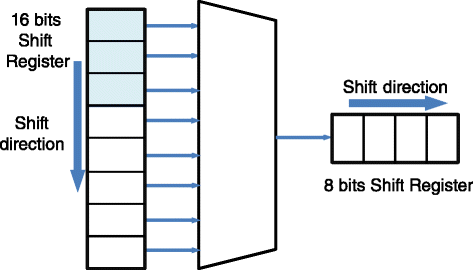
The idea behind the FR output stage
-
2)
The second approach consists, as shown in Fig. 11, of a shift register (SR) with parallel loading capabilities and an output register. The first register is a 24-bit up-down SR, while the output register is an 8-bit “normal” register. The Huffman code is loaded in the first register and then aligned to the contents possibly already present in the output register. Then, the code bits are transferred in parallel from the first register to the second. A finite state machine controls the alignment, the transferring, and the emission of a complete byte. A careful design of this control logic guarantees that the maximum number of shifts needed to perform the alignment is 4. The idea is simple: we can substitute a left shift operation with a shorter right shift operation. For example, a 6-bit shift on the left can be substituted with a 2-bit shift on the right. We will call this approach “SR output stage.”
Fig. 11 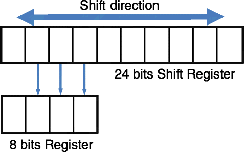
The idea behind the shifter output stages
-
3)
This approach is similar to the second. The only difference is that the 24-bit shift register is replaced by a 24-bit barrel shifter (BS). The control logic is almost the same as in the SR approach, and the limited number of shifts needed for the alignment reduces the complexity of this kind of shifter. We will call this approach “BS output stage.”


4 Simulation results
The developed model allows us to evaluate the performances (PSNR, clock cycles for encoding, latency…) of the system as a function of hardware parameters (such as the bit resolution of the fixed-point representation of the DCT data), or of parameters that can be reconfigured, such as the scan scheme or the length of restart intervals. Before considering these performances, we have to digress and consider a problem brought in by the restart interval mechanism. The length of the restart intervals affects obviously the compression time but also the compression factor, introducing a serious overhead problem.
First of all, we will consider this overhead problem introduced by the restart intervals. Then, we will examine the performances as a function of the reconfigurable and hardware parameters. Finally, we will present the results of the hardware implementation of the encoder. The compression efficiency strongly depends on the particular image to be compressed and on the correlation degree of its contents, so all the data presented in the graphs are an average over 20 images. In the simulations reported in Section 4.1, the color (YCbCr) images coming from the camera are 468 × 356 with 4:2:2 subsampling and 27-MHz sampling frequency. In Sections 4.2 and 4.3, we used, in order to speed up the simulations, smaller 64 × 32 images, keeping the subsampling and the sampling rate the same.
4.1 Restart markers overhead
The restart markers introduce an overhead in two ways. The first way is obviously the insertion of the 2 bytes of the markers themselves for each RST interval. This overhead is fixed: 2 bytes are introduced every n MCU, where n is the length of the restart interval, no matter how long is the encoded data for each MCU. The second way is the bit stuffing the encoder must insert before each RST marker. The JPEG standard requires that each marker segment to be byte-aligned, while the variable-length nature of the Huffman codes rarely produces this alignment. So, the encoder must insert fake bits before the markers, in order to byte-align the codestream. This insertion translates in an increase in the length of the encoded data. Obviously, the more are the restart markers (i.e., the shorter the restart interval length) and the more bits are wasted, and therefore, the lower is the compression efficiency.
The overhead as a function of the quality factor Q for different values of the restart interval and normalized to the length of the final byte stream is shown in Fig. 12. In the images used for these tests, the three components are grouped into a single scan. Observe how this overhead decreases increasing the restart interval length and increasing the quality factor. The former is the result we expected, the latter depends on the fact that increasing the quality factor increases the length of the whole codestream too, and so decreases the relative weight of the RST markers overhead.

Restart markers overhead as a function of the quality factor Q for different values of the restart interval length
This overhead depends also on the scan grouping. In a three-component image, four scan organizations are possible:
-
13: a single scan with all the three components
-
31: three scans with a single component each one
-
212: two scans with one component in the first scan and two in the second
-
221: two scans with two components in the first scan and one in the second
Figure 13 shows the overhead as a function of the restart interval for the different scan organizations; in this case, Q is equal to 50. As you can see, the overhead grows significantly with the number of scans, reaching a peak of more than 40 % in the case of three scans. The reason is related to the number of DUs that are in a MCU. Using a single scan with 4:2:2 subsampling, each MCU contains four DUs; using three scans each MCU contains one DU; hence, in the latter scheme, the number of restart markers is higher and therefore the overhead too.

Restart markers overhead as a function of the restart interval length for different scans grouping
This is a real problem. If we want to use the progressive transfer in a wireless network (that is if we want to send first the grayscale version of the image, and then later, if possible, the colors), we must use the 212 (first scan with grayscale and two colors in the second scan) or 31 (first scan with grayscale and the two colors in the second and third scan) coding. In this case, as can be seen from Fig. 13, the use of 212 is preferable to 31, due to the reduced overhead.
4.2 Encoder performance: clock cycles required for encoding
The overall performances depend heavily on the coding and on the DCT modules [8, 9, 11, 13]. However, the number of clock cycles of the coding depends on the image and on the quality factor Q, while the time required for the DCT is independent on these parameters. This is obvious, because the operations the DCT module needs to perform are always the same, while the encoding depends on how many coefficients it has to encode. If we are heavily quantizing the DCT coefficients, many of them will be almost zero, and they will be coded as a single coefficient. For example, if we have four zeros in a row, the encoder will produce a single encoded value. If we have four small—but not zero—DCT coefficients, the encoder will produce four different encoded values, and it will require many more clock cycles to end its duties.
This is clear from Fig. 14, that gives the number of clock cycles required to perform the JPEG encoding as a function of the quality factor, for the different architectures: the three output buffers and the FF and RAM approach to the DCT, described in previous section.

Number of clock cycles required to perform the JPEG encoding as a function of the quality factor
The three architectures for the output buffers, so different when the quality factor is maximum (when quantization is not used), rapidly become equivalent decreasing it. The lower the quality factor and the more correlated the image, the higher the compression ratio and therefore the smaller the size of the coded image. Therefore, the importance of coding tends to decrease with the quality factor, and the time required for the JPEG encoding is dominated by the DCT. Hence, reducing the quality of the compressed image, the number of clock cycles needed to perform the coding becomes less than the number of cycles needed to perform the DCT. When this happens, the coding module (and hence the output stage) spends a lot of time waiting for the ending of the DCT of a DU, and the time needed to compress a transformed DU is far less than the time needed to transform the next DU.
When the performances begin to be dominated by the DCT, the number of total cycles of the FF-DCT architecture becomes about 25 % lower than the RAM-DCT. The reason is that the latter takes two cycles to load the coefficients to be input to the arithmetic unit (adder/subtractor or multiplier, depending on the stage of the pipeline), while the former takes just one cycle to load both coefficients. To make a comparison, if the FF-DCT works at 60 MHz, the RAM-DCT must work at 75 MHz to reach the same throughput. This slowdown, though not excessive, is the price to pay for the savings in terms of logic resources obtained by the RAM-based architecture that will be shown in Section 4.3.
The consequence is that the best architecture depends strongly on the application. If we want to work with highly quantized (and compressed) images, the choice of the output stage is completely irrelevant, and we can choose the architecture that uses less hardware resources. From the DCT point of view, maybe we should use the faster architecture, even if it requires more resources. If we can tolerate that 25 % increase in the clock cycles number, however, we could keep using the RAM-DCT.
On the contrary, if we want to work with high-quality images, the DCT architecture choice is irrelevant, while the output stage becomes critical. In this case, we could save resources using the RAM-DCT and choose the faster (and more resource-consuming) output stage.
Let us consider now the dependency of the number of clock cycles required by the JPEG compression on the restart interval. We have seen in Fig. 14 that the number of clock cycles depends on the quality factor only for high Q and that the overhead due to the restart markers is low for high Q, as shown in Fig. 12.
Therefore, we expect that the number of clock cycles is almost independent from the length of the restart interval. This is confirmed in Fig. 15, which shows the number of clock cycles required to perform the JPEG encoding with Q = 100 as a function of the restart interval, for the different architectures for the output stage and for the DCT. Figure 15 reports the results of each one of the 20 images considered and the average value. The variability over the 20 images is relevant, but the number of clock cycles is almost independent on the length of the restart interval for each image and for the average value. The architecture that uses the Barrel shifter output stage requires less clock cycles to perform the compression.

Number of clock cycles required to perform the JPEG encoding as a function of the restart interval
Finally, we can consider the performance dependency on the scan scheme. This dependency is illustrated by Fig. 16. We can see in this figure how the number of clock cycles needed to compress an image is almost independent from the scan scheme chosen, while we might expect an increment in the clock cycles with the number of scans. The reason is that the pipeline used to create the offsets and the particular marker segments that bound the beginning of a scan hides the additional cycles needed to manage the scans. Therefore, in our architecture, neither the restart interval nor the scan mechanisms alter in any way the time needed to compress an image. As we will see in the next section, however, the scan mechanism comes with a significant need for hardware resources. Figure 16 reports the results of each one of the 20 images considered and the average value. As in Fig. 15, the variability over the 20 images is relevant, but the number of clock cycles is almost independent on the scan scheme for each image and for the average value. The architecture that uses the Barrel shifter output stage requires less clock cycles to perform the compression.

Number of clock cycles required to perform the JPEG encoding as a function of the scan scheme
4.3 Encoder performance: image quality versus number of bit in the fixed-point implementation
We talked about the quality of the image and about the so-called “quality factor.” Usually, the quality factor is an empirical parameter, between 1 and 100, which the user can choose in order to decide, in a heuristic way, the quality of the compressed image. This parameter is used to select a scaling factor that in turn can be used to scale all the quantization steps in the quantization matrices. The JPEG standard does not define a particular way to do this association—it is completely application dependent—so that the particular mathematical law used to extract the scaling factor is not important. The reasons behind the loss of quality in the compressed image are the quantization, which reduces the precision of the DCT coefficients, and the rounding errors in the calculation of the DCT and of the quantization. When the calculations are performed in floating-point arithmetic (i.e., in a C++ computer program), rounding errors can be neglected, and the image quality is dominated by the quality factor. When the calculations are performed with a dedicated hardware, however, they are usually implemented in fixed-point arithmetic, to simplify the circuitry. In this case, a key concern is the choice of the number of bits to be allocated for the data.
Now, the DCT applied to 8-bit samples produces coefficients that cannot require more than 11 bits for the integer part. The fast DCT we implemented, however, is a scaled version of the DCT standard row-column algorithm. In this scaled algorithm, several arithmetic manipulations are performed that isolate and collect the more multiplicative coefficients they can, and a single scaling coefficient is applied at the end of the calculations. These manipulations are done to reduce the number of multiplications and to speed up the final algorithm. Nevertheless, this implies that, even though the final precision (for the integer part) is 11 bits again, the intermediate calculations require a higher precision. Since the maximum scaling factor is 16, these intermediate calculations require 15 bits for the integer part. The choice of the number of bits of the fractional part will affect the quality of the final compressed image: obviously, the higher is the precision, the higher is the quality, but the higher is the complexity of the circuitry also. So it is important to find some kind of “optimum” precision, which minimizes the design complexity while keeping the highest as possible quality of the compressed image. A statistical description of the rounding errors and of the quantization noise in the DCT is presented in [27, 28], respectively.
The measure that is normally used for the measure of the quality of image processing is the PSNR:
where k is the number of bits representing each pixel and MSE is the mean square error, defined as
where n and m are the dimensions of the images and \( {I}_1 \) and \( {I}_2 \) are the images to be compared.
In order to find out this optimum, we evaluated the PSNR between an image compressed using floating-point arithmetic and an image compressed using fixed-point arithmetic, changing the precision of the fractional part. The higher is this PSNR, the more similar is the fixed-point image to the floating-point image. Figure 17 shows the PSNR as a function of the total number of bits (15 for the integer part and the rest for the decimal part) used for DCT and quantization with different quality factors. As we could expect, the quality falls down decreasing the precision of the calculations and the quality factor. When the Q is low and the precision is high, however, the quality of the image increases reducing the Q. The reason is that, when the Q decreases, the quantization masks the decrease in the precision of the calculations. This means again that the “optimum” we are looking for depends on what we want to do: if we want to work with highly compressed images, we can sacrifice arithmetic precision, obtaining almost the same quality but with less hardware resources. If we want to work with high-quality images, however, we have to use higher precision (and hence bigger) arithmetic circuits.

PSNR as a function of the resolution of the DCT and quantizer for different values of the quality factor Q
To be more specific, we investigated the relevance of the precision of the single modules DCT and quantization. In Fig. 18, obtained under the same conditions of Fig. 17, a smooth dependency of the PSNR on the accuracy in the calculations of the DCT is reported. The PSNR remains almost constant with precision down to 22 bits (with only 7 bits for the fractional part), and it remains quite high even at 19 bits (4 bits for the fractional part).

PSNR as a function of the resolution of the DCT for different values of the quality factor Q
For the choice of the optimum precision, we can use the PSNR of a compressed image obtained with floating-point calculations relative to the original image, shown in Fig. 19. The PSNR is 30 dB in the absence of quantization, when the image is compressed to its maximum quality and virtually indistinguishable from the original. So, a PSNR of 30 dB between a floating-point image and a fixed-point image means that the fixed-point image is virtually indistinguishable from the floating-point one. Therefore, using this value of 30 dB as a reference, we note that the PSNR in Fig. 16 is higher than 30 dB using 18 or more bits of precision (3 bits for the fractional part), which means that an image compressed using this reduced accuracy is substantially identical to an image compressed with floating-point arithmetic. To allow for a design margin, we can choose for example a 20-bit precision for the DCT calculations.

PSNR between floating-point compressed image and original image as a function of the quality factor Q
More delicate is the situation for the quantization. As shown in Fig. 20, the performances get worse rapidly decreasing the number of bits used for the quantizer, and this is more evident decreasing the quality factor. The reason is that the quantizer uses small coefficients and a multiplier to scale the DCT results. We preferred to use small coefficients and a multiplier instead of big coefficients and a divider because the divider circuits are very slow. However, if we encoded small coefficients with just a handful of bits, chances are that those coefficients would end up being almost zero, hence quantizing too heavily the DCT results. Using the same criterion seen for the precision of the DCT, we have to use more than 28 bits (thus reserving 13 bits for the fractional part). This is the precision we chose in our design for the quantization.

PSNR as a function of the resolution of the quantizer for different values of the quality factor Q
In summary, we can expect better performances by sacrificing the accuracy of the DCT, but keeping high the precision of the quantization, especially if our encoder is expected to work at low-quality factors.
4.4 FPGA implementation
Finally, we report, in Table 1, the results of the hardware implementation of the architecture in a Xilinx Virtex5 XC5VLX50T. The DCT arithmetic precision chosen is 20 bits, and the quantization precision chosen is 28 bits.
As mentioned in the literature [8, 9, 11, 13], for other architectures, the DCT_and_Quant module requires the greatest part of the resources. However, the decision to build the buffers with arrays of RAM instead of registers limits this occupation. In fact, a strong reduction of hardware resources is evident, comparing the results of the DCT block in Table 1 with Table 2, which reports the implementation of this module using flip-flops. This conclusion is emphasized by Table 3, which shows a comparison among our architectures and some previous works. It must be pointed out that all the architectures presented in the literature do not allow reconfigurability and restart interval and scan mechanisms. On the contrary, these features are allowed by the proposed architecture. Moreover, the DCT FF-architecture works at a lower frequency (79 MHz) with respect to the RAM-architecture (172 MHz). The FF-DCT can work at double frequency (158 MHz) introducing a two-level pipeline between the multiplier and the array of registers, but this will introduce an additional increment in hardware resources and latency. Essentially, using the RAM-DCT, we can get comparable frequency performances to those achievable with a double array of registers, but with an occupancy of logical resources far below.
Table 1 shows that the Scan_Manager is, surprisingly, the second block in terms of required resources. As we noticed in the previous section, the reconfigurability and the mechanism of the scans are responsible of the complexity of the Scan_Manager. Giving up the reconfigurability, we could also eliminate almost the entire block Init_JPEG, the fourth in terms of employment of logical resources. The block that inserts the restart markers, RST_Marker_Manager, however, requires only a small amount of resources.
The bottleneck for the maximum operating frequency is the Scan_Manager, and particularly the sub-module that takes care of initializing the scan, due to the presence inside it of a MAC used to calculate the number of DUs that fall in a restart interval. However, this is not a serious problem. The performances can be increased considering that this block is an initialization module and that it is executed only once per scan. So, we can speed up its operating frequency implementing the MAC with a shift-and-add approach: this will require more clock cycles to generate the restart interval, but this increment will be masked by the pipeline where the Scan_Manager works in. In fact, the scan initialization occurs while the Init_JPEG module is emitting the marker segments, and so before the compression can start.
The limit to 171 MHz in the quantizer is due to the multiplication of the quantization steps for the scaling factor during the module initialization phase. In our system, the Coordinator maintains the “base” quantization matrix and loads it into the quantizer making the steps to pass through a multiplier. Again, this is not a time-critical path, since the data are passed through only once during the initialization, and we could implement that multiplier with a shift-and-add approach, slower in terms of clock cycles, but faster if we look at the propagation delay.
As for the output stages, the two architectures that use up/down shifters (sliding or barrel) are those that require more resources, because the control state machine is far more complex that in the FR approach. The maximum frequency is higher in the case of shift registers, while the other is limited by the propagation delays. The maximum operating frequency of the FR approach is slightly lower than that of the BS approach.
Finally, in the encoder, there are several modules that work around 150 MHz. This limit is due to asynchronous accesses to small RAM inside them and can be increased simply making these accesses synchronous. Those RAMs are used as internal buffers to store coefficients while other modules are working: for example, to store DC coefficients while the AC coefficients encoding is still going. Making synchronous the access will simply add a clock cycle of latency.
5 Conclusions
In this paper, we designed a dedicate hardware implementation for FPGA of a JPEG encoder with high real-time reconfigurability, paying particular attention to the problems of wireless networks, i.e., the limited data rate and the sensitivity to noise.
With regard to the limited data rate, we made our encoder able to support different scans patterns, i.e., different groupings for the components of the input image. This allows, for example, to encode first the Y component of a YCbCr image, which is the grayscale version of the image, and therefore contains all the information necessary for its correct understanding, and then the chrominance components, that can be transmitted only when it is possible.
As for the noise protection, we added to the encoder the restart interval feature that makes the encoder able to recover from decoding errors introduced by the noise on a transmission channel.
In addition, we designed a completely reconfigurable system, through a series of buffers in the architecture, containing all the data necessaries for the compression and close to the modules that need to use them. These buffers can be changed on the fly depending on the requirements of the wireless channel. This can be useful for example to change the quality factor depending on the congestion of the network, or the length of the entire restart interval depending on the amount of noise measured on the network.
The project has been implemented on a Xilinx Virtex 5 FPGA. The architecture has been investigated in deep, and the performances in terms of overhead, latency, PSNR, hardware resources required, and maximum frequency for different values of the parameters of the architecture and of the JPEG standard parameters have been examined. Particularly, we implemented three different solutions for the output stage, and an architecture for the DCT module slightly slower than the fastest architecture we can find in literature, but far more resource-efficient.
We saw how the restart interval mechanism reduces the compression ratio of the final codestream, and we analyzed the dependency on the quality factor and on the scan scheme chosen. To reduce this overhead, the best solution is to keep the quality the highest as possible and to reduce the number of scans.
We saw then how the impact of the output stage architecture on the throughput is high when the quality is the highest and inexistent when the Q falls below 50. We saw also how the proposed DCT architecture is equivalent, from the throughput point of view to the solutions presented in the literature when the quality is the highest, and 25 % slower when the Q falls below 50. The throughput is moreover independent from the restart interval length and from the scan scheme chosen.
Finally, we analyzed the effect on the quality of the image of the fixed-point hardware precision used inside the DCT module. We saw how we can obtain better performances using a higher number of bits for the quantization and a lower one for the DCT.
References
GL Foresti, C Micheloni, L Snidaro, P Remagnino, T Ellis. (2005). Active video-based surveillance system: the low-level image and video processing techniques needed for implementation. IEEE Signal Processing Magazine 22(2), 25–37
Kleihorst R, Abbo A, Choudhary V, Schueler B. (2006). Design Challenges for Power Consumption in Mobile Smart Cameras, Proc. Cognitive systems with interactive Sensors (COGIS 2006).
M Bramberger, A Doblander, A Maier, B Rinner, H Schwabach. (2006). Distributed embedded smart cameras for surveillance applications. IEEE Computer Magazine 39(2), 68–75
Hengstler S, Prashanth D, Fong S, Aghajan H. (2007). MeshEye: a hybrid-resolution smart camera mote for applications in distributed intelligent surveillance, information processing in sensor networks (IPSN-SPOTS).
Pieretti A, Scavongelli C, Orcioni S, Conti M. (2010). Performance analysis of JPEG 2000 over 802.15.4 wireless image sensor network. Proc. of the IEEE 8th Int. Workshop on Intelligent Solutions in Embedded Systems, WISES10, pp. 55–60, Heraklion, Crete, Greece.
Conti M, Orcioni S. (2009). “Smart wireless image sensors for video surveillance”, in the book “Intelligent Technical Systems” Springer series“Lecture Notes in Electrical Engineering”, vol 38, pp.3-16
Santa-Cruz D, Grosboise R, Ebrahimi T. (2002). JPEG 2000 performance evaluation and assesment, Signal Processing: Image Communications, (17) 113–130.
Chen M, Chen T, Chen Y, Pan J, Weng Y. (1993). VLSI Implementation of Single Chip JPEG Codec, 1993 International Symposium on VLSI Technology, Systems and Applications, pp. 189–193.
Kovac M, Ranganathan N. (1995). JAGUAR: a fully pipelined VLSI architecture for JPEG image compression standard. Proceedings of the IEEE, 83(2), 247–258
S Sun, S Lee. (2003). A JPEG chip for image compression and decompression. Jurnal of VLSI Signal Processing 35, 43–60
Agostini L, Bampi S, Silva I. (2003). High throughput architecture of JPEG compressor for color images targeting FPGAs, 13th IEEE International Conference on Electronics, Circuits and Systems, pp. 180–183.
Quazi H, Qader F, Rasheed M, Mansoor H. (2005). An optimized architecture implementing the standard JPEG on FPGA, in Student Conference on Engineering Sciences and Technology.
Min K, Chong J. (2004). A real-time JPEG encoder for 1.3 megapixel CMOS image sensor SoC, 30th Annual Conference of the IEEE Industrial Electronics Society.
E Hamilton, (1992). JPEG file interchange format, v. 1.02
Reccomendation ITU-TT.81: Digital compression and coding of continuous-tone still images—requirements and guidelines, (1992)
Feig E, Winograd S. (1992). Fast algorithms for the discrete cosine transform. IEEE Transactions on signal Processing, 40(9), 2174–2193
Agostini L, Silva I, Bampi S. (2001). Pipelined fast 2-D DCT architecture for JPEG image compression, 14th Symposium on Integrated Circuits and Systems Design, pp. 226–231.
YT Chang, CL Wang. (1995). New systolic array implementation of the 2-D discrete cosine transform and its inverse. IEEE Transactions on Circuits and Systems for Video Technology 5(2), 150–157
TS Chang, CS Kunge, CW Jen. (2000). A simple processor core design for DCT/IDCT. IEEE Transactions on Circuits and Systems for Video Technology 10(3), 439–447
A Madanayake, RJ Cintra, D Onen, VS Dimitrov, N Rajapaksha, LT Bruton, A Edirisuriya. (2012). A row-parallel 8 × 8 2-D DCT architecture using algebraic integer-based exact computation. IEEE Transactions on Circuits and Systems for Video Technology 22(6), 915–929
YH Han, JJ Leou. (1998). Detection and correction of transmission errors in JPEG images. IEEE Transactions on Circuits and Systems for Video Technology 8(2), 221–231
R Chandramouli, N Ranganathan, SJ Ramadoss. (1998). Adaptive quantization and fast error-resilient entropy coding for image transmission. IEEE Transactions on Circuits and Systems for Video Technology 8(4), 411–421
S Orcioni, M Giammarini, C Scavongelli, GB Vece, M Conti. (2016). Energy estimation in SystemC with Powersim. Integration, the VLSI Journal-Elsevier 55(1), 118–128
Scavongelli C, Giammarini M, Conti M, Orcioni S. (2012). Computational cost estimation of a RTL JPEG architecture with Powersim, Proc. of the 10th Int. Workshop on Intelligent Solutions in Embedded Systems WISES 2012, Klagenfurth, Austria, pp. 9–14
Giammarini M, Orcioni S, Conti M. (2011). “Powersim: power estimation with SystemC: computational complexity estimate of a DSR front-end compliant to ETSI Standard ES 202 212”, Chap. 20 in the book “Solutions on Embedded Systems”, Springer Netherlands, series: Lecture Notes in Electrical Engineering, Dordrecht, pp. 285–300
Reccommendations ITU-R BT. 601–5—Studio encoding parameters of digital television for standard 4:3 and widescreen 16:9 aspect ratios.
ID Yung, SU Lee. (1993). On the fixed-point error analysis of several fast-DCT algorithms. IEEE Transactions on Circuits and Systems for Video Technology 3(1), 27–41
MA Robertson, RL Stevenson. (2005). DCT quantization noise in compressed images. IEEE Transactions on Circuits and Systems for Video Technology 15(1), 27–38
Competing interests
The authors declare that they have no competing interests.
Author information
Authors and Affiliations
Corresponding author
Rights and permissions
Open Access This article is distributed under the terms of the Creative Commons Attribution 4.0 International License (http://creativecommons.org/licenses/by/4.0/), which permits unrestricted use, distribution, and reproduction in any medium, provided you give appropriate credit to the original author(s) and the source, provide a link to the Creative Commons license, and indicate if changes were made.
About this article

Cite this article
Scavongelli, C., Conti, M. FPGA implementation of JPEG encoder architectures for wireless networks. J Embedded Systems 2017, 10 (2017). https://doi.org/10.1186/s13639-016-0047-5
Received:
Accepted:
Published:
DOI: https://doi.org/10.1186/s13639-016-0047-5