- Research
- Open access
- Published:
Symbolic execution and timed automata model checking for timing analysis of Java real-time systems
EURASIP Journal on Embedded Systems volume 2015, Article number: 2 (2015)
Abstract
This paper presents SymRT, a tool based on a combination of symbolic execution and real-time model checking for timing analysis of Java systems. Symbolic execution is used for the generation of a safe and tight timing model of the analyzed system capturing the feasible execution paths. The model is combined with suitable execution environment models capturing the timing behavior of the target host platform including the Java virtual machine and complex hardware features such as caching. The complete timing model is a network of timed automata which directly facilitates safe estimates of worst and best case execution time to be determined using the Uppaal model checker. Furthermore, the integration of the proposed techniques into the TetaSARTS tool facilitates reasoning about additional timing properties such as the schedulability of periodically and sporadically released Java real-time tasks (under specific scheduling policies), worst case response time, and more.
1 Introduction
Rigorous verification is essential for safety critical embedded hard real-time systems needing to comply with tight timing constraints. This is especially so for systems needing to comply with standards such as DO-178B, ISO-26262, IEC-61508, and EN-50128 applying to systems operating in safety-critical domains such as avionics and automotive. Of special interest is the verification of the system being schedulable, i.e., verifying that all real-time tasks under the conditions of the employed scheduling policy finish before their respective deadlines in all circumstances. The worst and best case execution time (WCET and BCET) often play an integral role in this relation—especially the former, which has applications in traditional methods for verification of schedulability such as response time analysis [1]. For systems written in (a suitable subset of) C, there are now many such analysis tools, both academic and commercial [2–10]. Most of these tools vary in the platforms they support, in the way they analyze programs and which restrictions they place on the analyzed programs, but as stated in [11] “To avoid having to solve the halting problem, all programs under analysis must be known to terminate. Loops need bounded iteration counts and recursion needs bounded depth.” The amount of required annotations is reduced by analysis, such as automatic loop-bound and array-call recognition.
1.1 Java for real-time system development
The Java programming language has recently received attention in the domain of real-time systems due to desirable characteristics, such as reduced development costs attributed to higher maintainability and productivity when compared to the C programming language, which for long has been the preferred choice in this domain.
However, Java in its traditional form is unsuitable for real-time systems for many reasons notably due to the inclusion of a (usually time unpredictable) garbage collector. To address this, the Java community, through JSR 302, has made tremendous progress and an important step has been taken with the upcoming Safety Critical Java (SCJ) profile [12] making Java a viable choice for development of embedded real-time systems. The SCJ profile introduces important real-time concepts such as high-resolution clocks and timers, but it also affects the programming model, e.g., by the introduction of a scoped memory model to avoid the need for a garbage collector. In addition, SCJ has a sufficiently tight thread semantics and a programming model based on tasks grouped in missions, all contributing to facilitating verification of real-time properties.
There are now several academic implementations of SCJ, including the OVM [13], HVM [14, 15], and Java Optimized Processor (JOP) [16]. The potential is also manifested in commercially available implementations [17–19] that have been used in industrial applications from the avionics domain, such as unmanned aircraft control systems [13], in the modernization of the Navy’s Aegis defense system [20], and in robot control [21].
There is a need in the real-time Java community for techniques and tools for temporal verification. Analyzing timing properties for Java programs is challenging primarily due to the fact that Java is usually translated to Java Bytecode, which is then interpreted by a Java virtual machine (JVM). This level of indirection complicates formal analysis as both program and JVM have to be taken into account for a given hardware platform; some of this complexity can, however, be reduced by a hardware implementation of the JVM such as JOP.
In recent years, several analysis tools for SCJ have been put forward including WCA [22], SARTS [23], TetaJ [24], and TETASARTS [25]. Characteristic for these is that they rely on reconstruction of the control-flow graph (CFG), which characterizes all possible execution paths of the program. This representation over-approximates possible program behavior since it also includes infeasible execution paths, i.e., execution paths for which there does not exist inputs that lead to that path being exercised. In turn, temporal behavior is over-approximated, thus likely yielding very pessimistic results of execution times that potentially affects the conclusions that can be made about the temporal correctness of the system—a system may be deemed unschedulable on a given platform although in reality it is schedulable.
1.2 Contributions
In this paper, we present a combination of symbolic execution [26, 27] and real-time model checking that generates a precise control-flow model from the symbolic execution trees obtained with a symbolic execution of the program. Each tree characterizes the set of feasible execution paths (up to some bound) of the analyzed task and yields a precise timing model. Both symbolic execution and model checking have issues with scalability due to the large number of paths respectively states to explore. We address this by using a “per task” symbolic execution leveraging the SCJ programming model that groups code into missions consisting of relatively short tasks. We will show experimentally using representative examples of real-time systems that our analysis approach is tractable.
The program model is built modularly. The timing behavior of the execution environment is obtained from environment models capturing the timing behavior of the JVM and hardware of the target platform. Based on a configuration, our technique generates the complete timing model as a network of timed automata (NTA) amenable to model checking using the UPPAAL [28] model checker. The NTA model can readily be used for estimating WCET and BCET but also generalizes to verification of properties expressible in timed computation tree logic (TCTL). In contrast to previous tools [24, 25], which provide limited feedback, our technique can also generate witness traces that expose the reported behavior, useful for debugging and program understanding.
Our technique is implemented as a tool, called JPF-SYMBC-RT, which can be used standalone for above purposes. The tool has also been integrated with the timing analysis tool TETASARTS—we will refer to this combination as the SYMRT tool. SYMRT is used for automatically constructing a complete timing model of Java real-time systems written in a variant of the SCJ profile. This model is similarly built on a per-task basis using JPF-SYMBC-RT, taking into account possible interference from other tasks. SYMRT allows to reason about additional timing properties such as the schedulability of periodically and sporadically released task, worst case response time (WCRT), worst case blocking time (WCBT), and processor utilization under the specified scheduling policy. SYMRT allows direct interaction with JPF-SYMBC-RT for conducting WCET and BCET analysis. To the best of our knowledge, SYMRT, and more specifically, the JPF-SYMBC-RT sub-component, is the first tool supporting BCET analysis of Java Bytecode. Both tools are open source; the project website http://people.cs.aau.dk/~luckow/symrt/ contains details on how to obtain the source code and usage instructions.
This paper presents SYMRT in terms of its design and capabilities and is organized as follows: in Section 2, we provide the preliminaries followed by Section 3, which discusses related work. Section 4 presents the overall design of SYMRT and its capabilities. We also show how the timing model is constructed using symbolic execution and real-time model checking in a task local approach and present optimizations for mitigating state space size. In Section 5, we present the usage of the tool along with experimental results. Section 6 contains conclusive remarks.
2 Background
2.1 Symbolic execution and SPF
Symbolic execution [26, 27] is a program analysis technique, which executes programs using symbolic inputs instead of concrete data. For each executed program path, a path condition is maintained, which represents the condition on the inputs for the execution to follow that path. The satisfiability of the path condition is checked using decision procedures and only feasible program paths are explored. A symbolic execution tree characterizes the explored paths. A program and its corresponding symbolic execution tree are shown in Fig. 1 a, b; a and b are symbolic values. We use this as a simple running example in the paper. Note that the execution path to line 4 is not included in the tree since the path condition a>b && a==b is unsatisfiable; hence, the corresponding conditional instruction in the tree does not branch. In contrast, a naïve CFG reconstruction would include this path. This particular infeasible path is likely to be identified and corrected during a code review, but let us note that for real-sized programs, they can be much more complex, e.g., due to semantic dependencies among several decision predicates, excluding manual identification as a viable technique.

a Running example. b Symbolic execution tree
Symbolic PathFinder (SPF) [29] is a symbolic execution framework built on top of the Java PathFinder (JPF) [30] model checking toolset for Java Bytecode analysis. SPF implements a Java Bytecode interpreter that replaces the standard execution semantics of Java Bytecodes with a non-standard symbolic execution. SPF handles dynamic input data structures (e.g., lists and trees) using lazy initialization [31]. Multi-threading is handled systematically using a form of partial order reduction from JPF. Symbolic execution of looping programs may result in an infinite symbolic execution tree; for this reason, SPF is run with a user-specified bound on the search depth. We will elaborate further on this in Section 4.
2.2 Timed automata
A timed automaton (TA) is a finite state machine extended with real-valued clocks and constraints on clocks. All clocks progress synchronously. A TA can be viewed as a graph; vertices are called locations and the arcs are called edges. Locations and edges have an associated set of clock constraints called invariants and guards, respectively. Invariants must hold when being in the location and time elapses. Guards must be satisfied to proceed to the next location. Edges are fired instantaneously and can reset a set of clocks.
A network of timed automata (NTA) is the parallel composition of a set of TAs. The TAs of an NTA proceed concurrently and communicate through synchronization channels and shared variables. Actions and co-actions on channels are denoted ! and ?, respectively.
In this paper, we will adopt an informal representation of TA corresponding to the GUI of UPPAAL; Fig. 2 shows an example and we use this to present informally the semantics of TAs. For a formal exposition of the semantics of TA and NTA, see, e.g., [32]. The TA contains three locations S0, S1 and S2 with S0 being the initial location. S0 has an invariant, y<=10, with y denoting a clock variable. The label, init(i), is a procedure, which will be called when the outgoing edge of S0 is fired. Its implementation is found in the declaration part of the TA definition. In S1, there are two outgoing edges labelled with guards y>=20 and y>50—they must be satisfied to fire the respective edge. S1 is also decorated with y ′==r u n[ i], a stop-watch expression (note the use of the apostrophe after the clock variable, here y), which starts or stops the clock depending on whether the right-hand side expression evaluates to true or false. r u n[ i] is an array and i is a parameter to the TA. S2 is a committed location; delays cannot occur and the next edge that will be fired must be an outgoing edge of a committed location. The outgoing edge of S2 is labelled with the action execute!; another TA is capable of synchronizing on it using execute?. The label y=0 is a clock reset.

UPPAAL timed automaton
3 Related work
3.1 WCET analysis tools
In recent years, a number of academic and commercial tools for static WCET analysis have been put forward; Ottawa [2], Chronos [3], Heptane [4], TuBound [5], SWEET [6], METAMOC [7], Bound-T [8], RapiTime [9], and the aiT WCET Analyzer [10]. Most of these tools are based on a three-step approach where a flow analysis provides information about possible execution paths, usually by constructing a CFG; a low-level analysis provides information about atomic operations on a given hardware platform; and a stage combining the flow analysis and timing of atomic operations is used to calculate the WCET. Many tools use the Implicit Path Enumeration Technique (IPET) (first introduced in [33]) which encodes the program as an integer linear programming (ILP) problem. The WCET can be estimated by solving the maximum cost circulation problem of the set of constraints that describes program behavior.
As C is the predominant programming language, most tools target this or binaries produced from C, e.g., the aiT WCET Analyzer. aiT is an abstract interpretation based state-of-the art industrial strength tool. The tool performs a per-task WCET analysis of binaries for a given execution platform taking the intrinsic cache and pipeline behavior into account. aiT also takes into account user annotations such as upper bounds on loop iteration counts, recursion depth, targets of indirect function calls, etc. The resulting WCET can be used as input for traditional schedulability analysis, however, as the aiT tool assumes that a task is executed sequentially and uninterrupted, it more or less prescribes a cyclic-executive schedule, as the tool assumes no interference.
Most of the mentioned tools analyze binaries, however, the SWEET [34] tool distinguishes itself by translating to ALF (Artist Flow Analysis language) and performs flow analysis on this representation. The result of the flow analysis is flow facts containing information about loop bounds and infeasible paths in the program. Such flow facts can be used as input for WCET tools such as RapiTime and aiT WCET Analyzer or the legacy low-sweet tool.
To compare WCET tools, the Mälardalen WCET Benchmarks [35] suite has been put forward and now includes a comprehensive overview of many of the above mentioned tools and their properties.
Many model-based timing analysis tools such as METAMOC [7] for executables, and WCA [22], TetaJ [24], SARTS [23], and TETASARTS [25] for Java rely on processing the program to build a CFG and enumerating the execution paths over the CFG. The paths are then translated to a modeling formalism, e.g., timed automata, and timing analysis is then formulated as a reachability problem using an appropriate logic such as TCTL. The temporal behavior of complex hardware features such as caches and pipelines can be modelled accurately as well. While these tools provide a safe approach, they are overly conservative, which is mostly a consequence of disregarding data in the reconstruction process.
3.2 Symbolic execution for timing analysis
An alternative to approximating execution paths using a CFG is symbolic execution [26, 27], which relies on a constraint solver to explore feasible paths. Symbolic execution has been explored before in the context of WCET analysis [36, 37], but neither presents a tool and the timing models are not used for the analysis of other temporal properties. However, [38] presents an integrated path and timing analysis method for C programs based on cycle-level symbolic execution using instruction-level simulation techniques. In six out of seven benchmarks, the method yields precise timings. Knoop et al. [39] presents a tool for WCET squeezing, which combines symbolic execution with IPET for computing a precise WCET bound. WCET Squeezing is an iterative post-process implemented in the r-TuBound [40] toolchain. It works by mapping the result of the IPET analysis to an execution trace in the program, which is then symbolically executed for determining the feasibility of the path. If it is infeasible, the ILP problem of IPET is extended with additional constraints that exclude that path from being considered again. The new ILP problem is then solved and the process starts over again. Thus, on each iteration, the WCET bound is made tighter.
The JPF toolset has been used before for the analysis of real-time Java. The work in [41] extends JPF’s explicit-state model checker to perform timing analysis. The approach uses discrete event simulation as a basis for modeling time. Another similar approach [42] is restricted for use with the JOP.
3.3 Schedulability analysis
Response time analysis [1] is a traditional approach for concluding on schedulability; the response times of the real-time tasks are calculated using WCET and blocking times, and the system is schedulable if the response times are less than the task deadlines.
TIMES [43] is a schedulability analysis tool using the NTA formalism. It is agnostic to the execution environment of the real-time system and relies on a specification of the tasks. SYMRT follows the approach of SARTS [23] and TETASARTS [25] relying on TIMES for its theoretical framework but, as opposed to TIMES, maintains a correspondence between the analyzed code and the model.
4 The SYMRT tool
SYMRT is built to accommodate the configuration of the execution environment in terms of hardware and JVM implementation. The latter can be a traditional, software implementation, such as the HVM, or a hardware implementation, such as the JOP. Parameters related to the temporal behavior of the system are configurable as well, such as the clock frequency of the hardware. The enabling technology for allowing timing analyses is model checking using UPPAAL. SYMRT and JPF-SYMBC-RT are open source and available from https://bitbucket.org/luckow/symrt/ and https://bitbucket.org/luckow/jpf-symbc-rt.
4.1 Overview
A high-level overview of SYMRT is shown in Fig. 3. SYMRT takes as input the Java class files constituting the real-time system and a configuration which, among others, specifies the analyses and the model generation technique. SYMRT allows the generation of two different timing models. The configuration specifies which model to generate, which can either be a complete timing model or an execution time analysis optimized model:
-
A complete timing model of the real-time system, which includes the real-time scheduling policy, all real-time tasks of the system and controllers for monitoring and controlling the state of the tasks. This timing model can be used for reasoning on schedulability, and facilitates analysis of WCET and BCET on task level, WCBT, and processor utilization and idle time. TetaSARTS is used with JPF-Symbc-rt for model extraction in this case.
Fig. 3 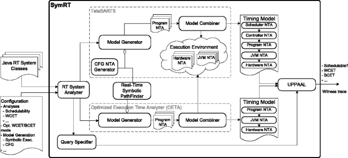
The architecture of SYMRT
-
An execution time analysis optimized model which needs not to reason on task interleavings and interactions, etc. Specifically, this model applies to the analysis of WCET and BCET, which by definition pertain to the unit of interest in isolation, i.e., the behavior of the remaining system is not taking into account. In addition, this model allows execution time analysis on method level. For generating this model, SymRT uses the Optimized Execution Time Analyzer (OETA) module which essentially offers direct interaction with JPF-Symbc-rt through the interface of SymRT.

Common to both generation techniques is the RT System Analyzer, which identifies the real-time tasks and extracts temporal scope information, e.g., release pattern, relative release point, and deadline, or, in case method level execution time analysis is specified, identification of this method information. Based on the configuration, the RT System Analyzer also forwards a specification of the target analyses to the Query Specifier, which constructs the UPPAAL queries accordingly. In summary, the target analyses for which SYMRT is currently envisioned are:
-
Schedulability analysis under the employed scheduling policy taking into account periodic (with offsets) and sporadic task releases, task interleavings, shared resources, and task blocking.
-
Analyzing the lowest possible clock frequency that still guarantees schedulability. This analysis can be used for improving the energy consumption of the system.
-
Processor utilization and idle time analysis (provided that the system is schedulable).
-
Worst case response time (WCRT) analysis similarly taking into account aforementioned task interference and blocking.
-
WCET and BCET analysis on task and method level.
All analyses are expressed in the specification language of UPPAAL, which extends TCTL. In essence, this means that the timing analyses supported by SYMRT are viewed as model checking problems. For example, the schedulability analysis is expressed as a reachability problem: the property of a non-schedulable system is expressed in TCTL and if the model, which is derived from the actual system, satisfies it, then we conclude also the system non-schedulable. The details on how the analyses are formulated are described later.
The model generator component in the TETASARTS module constructs the Program NTA by using either the original CFG NTA Generator or the Real-Time Symbolic PathFinder component. The former is based on reconstructing the CFG, while the latter is based on symbolic execution and works on the symbolic execution tree. The resulting Program NTA is then combined with the NTAs of the execution environment, i.e., the JVM NTA and the Hardware NTA, using the model combiner component. During this process, optimizations are also performed, e.g., for tailoring the JVM NTA to the hosting program. For details on the execution environment NTAs and optimizations, see [25, 44]. The product of the combiner is the complete timing model, which is amenable to model checking using UPPAAL, and the output will be the analysis result: for schedulability, it will be a yes/no answer, and for WCET a number. In addition, a witnessing trace, i.e., a sequence of symbolic states leading to the violating state, can be used for visualization and debugging.
The OETA module has similar major counterparts but does not reason on system level when generating the Program NTA. Using this module, it is possible to extract a trace leading to the WCET (and BCET) and visualize the respective execution paths. We will demonstrate this facility later in the paper.
4.2 Symbolic execution vs CFG-based model generation
Inevitably, considering all execution paths characterized by the CFG as in [7, 22, 24, 25] affects the analysis time, but it may also severely over-approximate the temporal behavior.
Virtual method invocations also complicate CFG-based approaches since all possible callees must be considered unless the reconstruction is complemented with additional analyses such as rapid type analysis [45] that attempts to reduce the set of possible callees. When using symbolic execution, SYMRT does not need to be complemented with such analyses, since the stack is part of the symbolic state, hence the callee is known at every call site of every execution path.
Additionally, in traditional CFG-based approaches, loop bounds are difficult to reason about and are usually either dealt with using annotations in the source code or through static analysis. Annotations are both prone to error and difficult to maintain. A related issue is nested loop structures with loop bound interdependencies, which are difficult to precisely incorporate in the timing model. Symbolic execution unrolls loops, hence, for most cases, neither loop bound annotations nor complementary loop bound analyses are necessary (see Section 5 for examples) except when the bound is dependent on, for example, I/O or the unrolling exceeds the specified analysis depth. In cases where annotations are necessary, SYMRT offers (simple) comment-based loop bound annotations on the form //@loopbound = bound; SYMRT will unroll the loop up to the specified bound and explicitly break it. To represent input values from, e.g., sensory equipment, we introduce a symbolic variable. If the search depth limit of symbolic execution is reached, the resulting timing model will only be correct up to that bound, and hence SYMRT issues a warning. The search depth can then be increased.
4.3 Model construction
The JPF-SYMBC-RT component of SYMRT conducts a post-translation of the symbolic execution tree to the NTA formalism using a newly developed symbolic execution tree capability available in JPF-SYMBC V7 [46].
Capturing the temporal behavior of the execution paths of the real-time tasks is done at Java Bytecode instruction level; for each Java Bytecode of the execution path, a location is created in the TA and connected by outgoing edges to successor locations corresponding to the control flow. For branching instructions, such as IFEQ and FCMPL, there can be up to two and three outgoing edges, respectively, if the path conditions of the branches are satisfiable (or if the decision procedure is inconclusive). For all other instructions, there will be only one outgoing edge.
The translation process distinguishes between how the execution environment timing model is provided:
-
1.
The timing model can be provided as fixed execution times or as intervals for all the (supported) Java Bytecodes using a timing scheme. Elaborating on the construction of timing schemes is beyond the scope of this paper, but let us note here that they can either be constructed by a careful measurement-based method or by using static analysis of the implementation as in our related work in [47].
-
2.
The timing model is directly encoded as an NTA itself, i.e., the temporal behavior of each Java Bytecode is simulated including the hardware state as determined by, e.g., caching and pipelining. This approach has the potential of yielding a more precise timing model than the translation approach 1, because the temporal behavior of each Java Bytecode is not regarded as an interval but actual simulations. For example, this will more precisely capture the effect of a shared pipeline and cache when tasks are scheduled. The potential benefits of this approach come at the expense of a bigger state space, and currently only small, although realistic, applications, such as the Minepump control system [1, 24], are tractable for analysis.
Figures 4 and 5 show excerpts of the two modeling approaches for an imaginary instruction instr1.

Translation to TA corresponding to translation 1

Translation to TA corresponding to translation 2
In Fig. 4, each location encodes as an invariant the timing constraints of the corresponding instruction: e x e c u t i o n T i m e≤W C E T_i n s t r1 specifies that the system can at most spend the WCET of instruction instr1 in that location. The stop-watch expression e x e c u t i o n T i m e ′==r u n n i n g[ t I D] ensures that the clock is only progressing when the task to which this particular TA belongs is running as governed by the scheduling policy. In case the analysis is targeted solely at execution time analysis, the stop-watch expression is omitted. The guard ensures that the execution time of instr1 is simulated for at least its BCET. Both the WCET and the BCET are obtained from a timing scheme describing the temporal behavior of all the supported Java Bytecodes on the target execution environment (configuration of JVM and hardware).
For this translation approach, JPF-SYMBC-RT employs state reduction on non-breakable, sequentially executed instructions in the NTA inspired by [25]. Sequentially executed instructions are not branching and all instructions except monitor instructions and invocations yielding the firing of a sporadic event are non-breakable. Let E l denote the execution time of the instruction represented by location l. When the instruction execution times are known, the total execution time of n sequentially executed instructions represented by locations l 1,l 2,…,l n , is \(E_{\{l_{1},l_{2},\ldots,l_{n}\}} = {\sum \nolimits }_{i=1}^{n}E_{l_{i}}\). Thus, this sequence can be replaced by a single location with execution time \(E_{\{l_{1},l_{2},\ldots,l_{n}\}}\). For a bubble sort algorithm, the number of locations before and after the optimization is 163,549 and 1441, respectively, thus reducing 99.1 % of the locations. Effectively, the optimization yields a control flow representation of the basic blocks constituting the feasible paths as determined by symbolic execution. Figure 6 shows the TA (after applying optimizations) of the running example.

TA after state reduction
JPF-SYMBC-RT also uses progress measures; a variable in the model that is incremented to describe progress in the model. When all traces corresponding to a specific value of the progress measure have been crossed, the memory of previous states can be removed, thus reducing overall memory consumption of the analysis.
The product of translation approach 2, shown in Fig. 5, relies on simulating the execution time based on the state of JVM and the hardware. Separate NTAs are used for capturing the timing behavior of the program, the JVM and the hardware, denoted the Program NTA, the JVM NTA, and the Hardware NTA, respectively. The interactions among them capture the dependencies between the temporal behavior, e.g., the temporal properties of an arbitrary Java Bytecode modelled in the JVM NTA is dependent on the pipeline and cache state of the processor in the Hardware NTA. The interactions are well-defined using dedicated (co-)actions and shared variables, making it possible to replace NTA components to configure the analysis to the desired execution environment.
During the process of combining the Program NTA generated by JPF-SYMBC-RT with the JVM NTA and the Hardware NTA, optimizations are performed, e.g., for tailoring the JVM NTA to the hosting program. For details on the execution environment NTAs and optimizations, see [25, 44, 47].
In [47], we have shown how a JVM NTA can be derived directly from the HVM executable. Here, it suffices to say that the instruction is passed to the JVM NTA by the jvm_instruction shared variable. jvm_execute! initiates the simulation in the JVM NTA. For JOP, SYMRT allows simulating exactly variable block FIFO, FIFO, and LRU method cache replacement policies. The simulation approach is similar to that used in WCA [22].
An example of a Hardware NTA is shown in Fig. 7.

Hardware TA models from METAMOC [7]. a Pipeline fetch stage. b Pipeline execute stage
Here, the combination of the fetch channel and asm_inst establishes the communication link with the JVM NTA. The JVM NTA synchronizes on the channel whenever a machine code instruction (as provided by the asm_inst variable) is to be simulated (in this case directly put into the fetch stage of the pipeline). The machine instruction will be simulated for [best_wait;worst_wait] time.
The product regardless of whether translation approach 1 or 2 is used is the complete timing model with the analyses specified as UPPAAL specifications. The output of model checking is the analysis result, e.g., a yes/no answer for TCTL properties, and a number for WCET and BCET analysis. In addition, for execution time analysis, a witnessing trace, i.e., a sequence of symbolic states leading to the violating state, can be used for debugging, visualization, and program understanding.
4.4 Per-task analysis
The timing model of a multi-tasking real-time system is built modularly, based on the symbolic execution of each individual task. Whenever an instance or a static variable is read (via GETFIELD or GETSTATIC bytecodes), the per-task analysis checks to see if the variable is possibly shared among multiple tasks. A variable is shared if it is referenced in a chain of references from a static field or from a task (thread) object. SYMRT also relies on additional checks in JPF for determining sharedness, e.g., if the field is immutable. We have implemented a procedure that propagates the sharedness information along reference chains whenever an update happens (via PUTFIELD and PUTSTATIC) to a variable that was marked as shared. Furthermore, the lazy initialization used in handling symbolic references has also been modified to mark all the newly created objects as shared (if the symbolic fields belong to a shared object).
If the variable is considered shared, a safe modular generation of the timing model for the task must account for values written to that variable from other tasks. This is necessary, because the values may alter the control flow of the logic in the task and possibly make feasible other execution paths that may yield a higher WCET (or lower BCET) thus rendering the analysis unsafe if these are not considered. To account for this, the per-task analysis automatically introduces fresh symbolic variables for the potentially shared variables. Hence, these accounts for all possible values that can be assigned to the shared variables and therefore captures all possible thread interferences. This yields a safe local analysis of the tasks because the symbolic variables over-approximate the values of shared variables and thus the feasible execution paths.
Generating timing models for each task using this per-task analysis significantly reduces the complexity of symbolic execution because any behavior of the system outside the local task needs not to be considered. The composition of all timing models generated from the tasks from the per-task analysis yields a complete system model which is also safe, because the composed model over-approximates the possible interference between the tasks.
4.5 Model analysis
When JPF-SYMBC-RT is used directly for execution time analysis, the TA shown in the screenshot in Fig. 8 of the running example is generated. WCET and BCET can be determined using the sup-query (inf-query) extensions of UPPAAL, which determine the supremum (infimum) value of the specified clock(s). WCET and BCET can be formulated as s u p{f i n a l}:e x e c u t i o n T i m e and i n f{f i n a l}:e x e c u t i o n T i m e, respectively. Note also that the simulator is capable of visualizing the trace (i.e., sequence of states) leading to the (in this case) WCET of the program.

Screenshot of UPPAAL
For a complete timing model, the NTA is further extended with TAs from TETASARTS capturing the scheduling policy and for controlling and monitoring the state of associated real-time tasks. A controller for periodic tasks is shown in Fig. 9. Controllers for sporadic tasks are similar except that their eligibility for being scheduled is determined by the previous firing of the associated event. The task TAs are modified for making the association to a corresponding controller resulting in the TA shown in Fig. 10 for our running example.

TA controlling a periodic task

TA for the task when using a complete timing model
The connection is created using the run[tID] channel; tID is a task identifier. Note that the values of offset, deadline, and period are extracted from the task instantiations in the source code. Clock variables corresponding to the target analyses are generated as part of the controller TA, hence enabling WCET, WCRT, and WCBT analyses in this example using the same timing model. The controller TA will enter the ExecutingThread location when the associated task is executing. The clock releasedTime is used to track the relative time from the release point. If it exceeds the deadline of the task, the DeadlineOverrun location is entered, otherwise execDone is entered and the process continues when the period is met.
The analyses are conducted by viewing them as reachability problems expressible in temporal logic; we can formulate schedulability analysis as: is it possible to reach a state where a task misses its deadline? This state is represented by the location DeadlineOverrun previously mentioned. Assume a system composed of n tasks T i with corresponding DeadlineOverrun i locations in the controllers for i∈{1,2,…,n} and let \(\phi = \bigvee _{i} DeadlineOverrun_{i}\) denote the disjunctive state formula of the DeadlineOverrun locations. Schedulability analysis can then be expressed as A□ n o t ϕ, i.e., in all reachable states, ϕ is not satisfied.
For the other supported analyses, we use sup- and inf-queries. WCET and BCET analysis can be conducted using sup{TC.ExecutingThread}:TC.wcet and inf{TC.Done}:TC.wcet, respectively, where TC is the task controller of the real-time task. Note in Fig. 9, that the wcet clock is only progressing when the task is set for execution due to the stop-watch expression. WCRT and WCBT analysis can be conducted using s u p{T C.E x e c u t i n g T h r e a d}:T C.w c r t and s u p{T C.E x e c u t i n g T h r e a d}:T C.b l o c k i n g T i m e, respectively. Note that the blockingTime clock is only progressing when the task is blocked. Processor utilization and idle time analysis can be conducted by introducing a new TA with a single location with the stop-watch expression u t i l ′ == !i d l i n g && i d l e ′ == i d l i n g where util and idle are two new clock variables and idling a boolean variable that is set whenever a task is executing. A sup-query on util and idle clocks is used for the analyses.
5 Experimental results
We first introduce a comparison of the WCET and BCET estimates obtained from SYMRT (using directly JPF-SYMBC-RT) and the state-of-the-art in execution time analysis for Java real-time systems. To the best of our knowledge, WCA tool is the only tool that supports WCET analysis for Java Bytecode besides TETASARTS and SYMRT. In addition, we do not know of any other tool that supports automated schedulability analysis of Java Bytecode, except TETASARTS and it predecessor, SARTS. Furthermore, we are not aware of other tools for analysis of additional temporal properties such as BCET and WCRT of Java Bytecode. We have used as examples the Java implementations (obtained from the JOP distribution1) of a subset of the algorithms from the Mälardalen WCET benchmark suite [35]: binary search (54 LOC), bubble sort (34 LOC), quick sort (109 LOC), insertion sort (39 LOC), iterative Fibonacci (40 LOC), and select smallest (137 LOC) which selects the nth smallest number in an array. For the sorting algorithms, the array is initialized with symbolic values. For binary search, the search key is symbolic. For Fibonacci, the input value, n, is symbolic and constrained such that 1≤n≤30. For select smallest, an array of size 20 is filled with concrete values. The search key is symbolic and bounded by the array length. Note that we did not need to provide loop bound annotations in any of the examples nor did we reach the default search depth (corresponding to 100 branches) during analysis.
We have used two configurations of the execution environment; (1) JOP and (2) HVM2 [48] running on the AVR ATmega2560. The timing model of the latter is a generated Timing Scheme. We use the same configuration of the execution environment across the tools, e.g., SYMRT and WCA have been configured with read and write wait cycles set to 1 and 2 (and cache configuration is the same). Also, to give indications of the precision of SYMRT, we compared with measurements of BCET and WCET obtained by using inputs yielding the best and worst case behavior (e.g., for bubble sort, a sorted and unsorted list). We used the JOP simulator to read the cycle count before the first instruction is executed of the target method and after the return instruction. For HVM+AVR, the measurements have been obtained in a similar way by using the debugging facilities of Atmel Studio 6. For this set of experiments, we used a laptop with an Intel Core i7-2620M CPU @ 2.70 GHz with 8 GB of RAM. The peak memory consumption for symbolic execution is 500–700 MB for all examples. UPPAAL peaks at 50–200 MB during model checking. Table 1 shows the results for the comparison on JOP.
First note that all estimates indicate safety, that is BCET symrt ≤BCETm and WCET symrt ≥WCETm and that the precision of SYMRT is better (and in two cases equally as good) as the other tools. The major contributor to the pessimistic results of TETASARTS and WCA are that they over-approximate the iterations of nested loops with interdependencies. The analysis time using SYMRT is however longer, which is due to symbolic execution. This is as expected, because WCA relies on analyzing the static structure of the program as CFG, which can relatively quickly be reconstructed. Model checking time is negligible for SYMRT and WCA.
Also note that for quick sort, it is relatively difficult to exercise and measure the path yielding the worst case behavior since it depends on the pivot element selection.
Table 2 shows the comparison on HVM and AVR ATmega2560. Again, all estimates produced by SYMRT are safe and more precise than TETASARTS. For this first set of experiments (including the results obtained for JOP), the analysis time is largely attributed symbolic execution. In all cases, model checking using UPPAAL takes less than a second.
We compare the schedulability analysis of SYMRT with TETASARTS using the Minepump control system [1, 24] (0.5 KLOC), the real-time sorting machine (RTSM) [23] (0.3 KLOC) and a variant of MD5SCJ [25] with multiple tasks (0.4 KLOC). We also conducted the analysis on the MER Arbiter (3.6 KLOC) that models a flight software component for the Mars Exploration Rover (MER) developed at NASA JPL [49]. It was not written for real-time Java, but it features two users that use a number of resources; we made a minor revision associating to each user a periodic handler. Finally, we also analyzed a version of the Lift real-time system from Jembench [50] with 18 tasks. TETASARTS has not been able to construct the models for MER and Lift. Even though MER is relatively simple, the dependency extent computed in TETASARTS for generating the CFG is too large.
Clearly, there are systems for which analysis is intractable. This is for instance the case when attempting to do a full schedulability analysis for the MER on HVM on the AVR processor when a precise execution environment model is used. However, note that the limitations of the analysis are not determined by the number of lines of code. It is rather the number of branches that need to be exercised, along with the number of tasks, that determines the limitations as the size of the UPPAAL model grows exponentially with the number of components in the NTA. However, since schedulability is viewed as a reachability problem, it may be possible to translate it into the subset of the UPPAAL modeling language supported by the opaal+LTSmin system [51]. In [52], opaal+LTSmin demonstrates a speedup of 40 on a 48 core machine compared to UPPAAL. Future work will investigate this direction.
The TS subscript denotes that a timing scheme with fixed execution times for all the Java Bytecodes has been used instead of modeling their behavior as an NTA. For this set of experiments, we used an application server with an Intel Xeon X5670 @ 2.93 GHz CPU and 32 GB of RAM. The results are shown in Table 3.
In all cases, the systems have been deemed schedulable, and the results show that the analysis times and memory consumptions are lower when using SYMRT. We also tried, e.g., RTSM with HVM+AVR, but the complexity of the resulting models, regardless of the tool used is too big, which can be attributed the JVM NTA, which largely dominates the complexity. In this case, UPPAAL runs out of memory.
6 Conclusions
We have presented SYMRT, a timing analysis tool that uses a combination of symbolic execution and model checking to achieve flexible and tight verification of timing properties of real-time Java systems. We have elaborated on the translation of the symbolic execution tree to the NTA modeling formalism of UPPAAL enabling a modular and configurable system timing model.
We have shown that SYMRT can produce BCET and WCET estimates that in most cases are more precise than state-of-the-art in real-time Java. These results are in line with findings for C-like programs [38]. A tight execution time estimate is paramount for concluding on schedulability and SYMRT facilitates schedulability analysis by using the techniques from TETASARTS. As the interactions between tasks are taken into account during schedulability analysis, systems deemed unschedulable using traditional response time analysis may be deemed schedulable using model checking as demonstrated in [23]. SYMRT also allows the clock frequency of the target hardware to be set prior to the analysis, thus making it possible to determine the lowest clock frequency at which the system is still schedulable as demonstrated in [44].
It is perhaps surprising that the combination of symbolic execution and model checking works so well as both have issues with scalability due to the large number of paths respectively states to explore. However, by using a “per task” symbolic execution leveraging the Safety Critical Java (SCJ) programming model that groups code into missions consisting of relatively short tasks, the analysis is tractable. Furthermore, when using timing models of the target execution environment, the generated TA of the program is at basic block level, which significantly reduces the state space size.
We are working on applying SYMRT for the performance analysis of different components of the NASA tactical layer solution for planes, T-TSAFE, currently focusing on the conflict detection and conflict resolution algorithms.
7 Endnotes
1 Available for download at http://www.jopdesign.com/
2 Available for download at http://icelab.dk/
References
A Burns, A Wellings, Real-time systems and programming languages: ADA 95, real-time Java, and real-time POSIX, 4th (Addison-Wesley Educational Publishers Inc., Boston, MA, USA, 2009).
C Ballabriga, H Cassé, C Rochange, P Sainrat, in Software Technologies for Embedded and Ubiquitous Systems, ed. by S Min, R Pettit, P Puschner, and T Ungerer. OTAWA: an open toolbox for adaptive WCET analysis (SpringerBerlin, Heidelberg, 2010), pp. 35–46. doi:10.1007/978-3-642-16256-5_6
X Li, Y Liang, T Mitra, A Roychoudhury, Chronos: a timing analyzer for embedded software. Sci. Comput. Program. 69(1), 56–67 (2007).
A Colin, I Puaut, in Real-Time Systems, 13th Euromicro Conference On. A modular and retargetable framework for tree-based WCET analysis (IEEE, 2001), pp. 37–44.
A Prantl, M Schordan, J Knoop, in 8th International Workshop on Worst-Case Execution Time Analysis (WCET’08), OpenAccess Series in Informatics (OASIcs), 8, ed. by R Kirner. TuBound - a conceptually new tool for worst-case execution time analysis (Schloss Dagstuhl–Leibniz-Zentrum fuer InformatikDagstuhl, Germany, 2008). doi:10.4230/OASIcs.WCET.2008.1661. also published in print by Austrian Computer Society (OCG) with ISBN 978-3-85403-237-3. http://drops.dagstuhl.de/opus/volltexte/2008/1661. Accessed 23 Sep 2015.
MUR-TR Center, SWEET (SWEdish Execution Time tool). http://www.mrtc.mdh.se/projects/wcet/sweet/. Accessed 23 Sep 2015.
AE Dalsgaard, MC Olesen, M Toft, RR Hansen, KG Larsen, in 10th International Workshop on Worst-Case Execution Time Analysis. METAMOC: modular execution time analysis using model checking, (2010). doi:http://dx.doi.org/10.4230/OASIcs.WCET.2010.113. http://drops.dagstuhl.de/opus/volltexte/2010/2831. Accessed 23 Sep 2015.
N Holsti, S Saarinen, in Space Syst. Finl. Ltd. Status of the Bound-T WCET tool, (2002), pp. 25–30. Euromicro.
RapiTime, RapiTime WCET tool homepage. Website. http://www.rapitasystems.com. Accessed 23 Sep 2015.
C Ferdinand, R Heckmann, B Franzen, in Proceedings of VVSS2007 - 3rd European Symposium on Verification and Validation of Software Systems, 23rd of March 2007, Eindhoven, ed. by P Groot. Static memory and timing analysis of embedded systems code, (2007). http://www-fp.cs.st-andrews.ac.uk/embounded/pubs/papers/VVSS07.pdf. Accessed 23 Sep 2015.
R Wilhelm, D Grund, Computation takes time, but how much?Commun. ACM. 57(2), 94–103 (2014). doi:http://dx.doi.org/10.1145/2500886
D Locke, BS Andersen, B Brosgol, M Fulton, T Henties, JJ Hunt, JO Nielsen, K Nilsen, M Schoeberl, J Tokar, J Vitek, A Wellings, Safety-Critical Java Technology Specification, Public Draft, (2013). Java Community Process http://www.jcp.org/en/jsr/detail?id=302. Accessed 23 Sep 2015.
A Armbruster, J Baker, A Cunei, C Flack, D Holmes, F Pizlo, E Pla, M Prochazka, J Vitek, A real-time Java virtual machine with applications in Avionics. ACM Trans. Embed. Comput. Syst. (TECS). 7(1), 5–1549 (2007). doi:http://dx.doi.org/10.1145/1324969.1324974
S Korsholm, Java for cost effective embedded real-time software (Department of Computer Science, Aalborg University, 2012).
KS Luckow, SE Korsholm, B Thomsen, in Proceedings of the 23rd Nordic Workshop on Programming Theory. NWPT ’11. Towards a real-time, WCET analysable JVM running in 256 kB of flash memory, (2011), pp. 68–88. www.mrtc.mdh.se/nwpt2011/nwpt11-proceedings.pdf. Accessed 23 Sep 2015.
M Schoeberl, JOP: A Java Optimized Processor for Embedded Real-Time Systems, vol. ISBN 978-3-8364-8086-4 (VDM Verlag Dr. Müller, 2008). http://www.amazon.com/JOP-Optimized-Processor-Embedded-Real-Time/dp/3836480867. Accessed 23 Sep 2015.
F Pizlo, L Ziarek, J Vitek, in Proceedings of the 7th International Workshop on Java Technologies for Real-Time and Embedded Systems. JTRES ’09. Real time Java on resource-constrained platforms with Fiji VM (ACMNew York, NY, USA, 2009), pp. 110–9. doi:http://dx.doi.org/10.1145/1620405.1620421. http://doi.acm.org/10.1145/1620405.1620421. Accessed 23 Sep 2015.
Aicas, JamaicaVM user manual: Java technology for critical embedded systems (2010).
Atego, Atego home (2013). http://atego.com/. Accessed 23 Sep 2015.
K Nilsen, in Proceedings of the 2012 ACM Conference on High Integrity Language Technology. HILT ’12. Real-time Java in modernization of the aegis weapon system (ACMNew York, NY, USA, 2012), pp. 63–70. doi:10.1145/2402676.2402699. http://doi.acm.org/10.1145/2402676.2402699. Accessed 23 Sep 2015.
SG Robertz, R Henriksson, K Nilsson, A Blomdell, I Tarasov, in Proceedings of the 5th International Workshop on Java Technologies for Real-time and Embedded Systems. JTRES ’07. Using real-time Java for industrial robot control (ACMNew York, NY, USA, 2007), pp. 104–110. doi:http://dx.doi.org/10.1145/1288940.1288955. http://doi.acm.org/10.1145/1288940.1288955. Accessed 23 Sep 2015.
M Schoeberl, W Puffitsch, RU Pedersen, B Huber, Worst-case execution time analysis for a Java processor. Softw. Pract. Experience. 40(6), 507–542 (2010). doi:10.1002/spe.968
T Bøgholm, H Kragh-Hansen, P Olsen, B Thomsen, KG Larsen, Model-based schedulability analysis of safety critical hard real-time Java programs (2008). doi:10.1145/1434790.1434807. http://doi.acm.org/10.1145/1434790.1434807. Accessed 23 Sep 2015.
C Frost, CS Jensen, KS Luckow, B Thomsen. 9th International Workshop on Java Technologies for Real-Time and Embedded Systems, (2011). doi:10.1145/2043910.2043916. http://doi.acm.org/10.1145/2043910.2043916. Accessed 23 Sep 2015.
KS Luckow, T Bøgholm, B Thomsen, KG Larsen, in Proceedings of the 11th International Workshop on Java Technologies for Real-time and Embedded Systems. JTRES ’13. TetaSARTS: a tool for modular timing analysis of safety critical Java systems (ACMNew York, NY, USA, 2013), pp. 11–20. doi:10.1145/2512989.2512992. http://doi.acm.org/10.1145/2512989.2512992. Accessed 23 Sep 2015.
JC King, Symbolic execution and program testing. Commun. ACM. 19(7), 385–394 (1976).
LA Clarke, A system to generate test data and symbolically execute programs. IEEE Trans. Softw. Eng. 2(3), 215–222 (1976).
J Bengtsson, K Larsen, F Larsson, P Pettersson, W Yi, in Proceedings of the DIMACS/SYCON Workshop on Hybrid Systems III : Verification and Control: Verification and Control. Uppaal – a tool suite for automatic verification of real-time systems (SpringerSecaucus, NJ, USA, 1996), pp. 232–243. http://dl.acm.org/citation.cfm?id=239587.239611. Accessed 23 Sep 2015.
CS Păsăreanu, W Visser, D Bushnell, J Geldenhuys, P Mehlitz, N Rungta, Symbolic PathFinder: integrating symbolic execution with model checking for Java bytecode analysis. Autom. Softw. Eng. 20(3), 391–425 (2013). doi:http://dx.doi.org/10.1007/s10515-013-0122-2
JPF, Java PathFinder tool-set (2014). http://babelfish.arc.nasa.gov/trac/jpf. Accessed 23 Sep 2015.
S Khurshid, CS Păsăreanu, W Visser, in Proceedings of the 9th International Conference on Tools and Algorithms for the Construction and Analysis of Systems. TACAS’03. Generalized symbolic execution for model checking and testing (SpringerBerlin, Heidelberg, 2003), pp. 553–568. http://dl.acm.org/citation.cfm?id=1765871.1765924. Accessed 23 Sep 2015.
J Bengtsson, W Yi, in Lectures on Concurrency and Petri Nets, Lecture Notes in Computer Science, 3098, ed. by J Desel, W Reisig, and G Rozenberg. Timed automata: semantics, algorithms and tools (Springer, pp. 87–124. doi:10.1007/978-3-540-27755-2_3. http://dx.doi.org/10.1007/978-3-540-27755-2_3. Accessed 23 Sep 2015.
Y-TS Li, S Malik, in Proceedings of the 32Nd Annual ACM/IEEE Design Automation Conference. DAC ’95. Performance analysis of embedded software using implicit path enumerationACMNew York, NY, USA, 1995), pp. 456–461. doi:10.1145/217474.217570. http://doi.acm.org/10.1145/217474.217570. Accessed 23 Sep 2015.
J Gustafsson, A Ermedahl, C Sandberg, B Lisper, in Real-Time Systems Symposium, 2006. RTSS’06. 27th IEEE International. Automatic derivation of loop bounds and infeasible paths for wcet analysis using abstract execution (IEEE Computer SocietyWashington, DC, USA, 2006), pp. 57–66. doi:http://dx.doi.org/10.1109/RTSS.2006.12
J Gustafsson, A Betts, A Ermedahl, B Lisper, in Proceedings of the 10th International Workshop on Worst-Case Execution Time Analysis. The Mälardalen WCET benchmarks—past, present and future, (2010). http://www.es.mdh.se/publications/1895-. Accessed 23 Sep 2015.
D Kebbal, P Sainrat, in 6th International Workshop on Worst-Case Execution Time Analysis (WCET’06), OpenAccess Series in informatics (OASIcs), 4, ed. by F Mueller. Combining symbolic execution and path enumeration in worst-case execution time analysis (Schloss Dagstuhl–Leibniz-Zentrum fuer InformatikDagstuhl, Germany, 2006). doi:http://dx.doi.org/10.4230/OASIcs.WCET.2006.675. http://drops.dagstuhl.de/opus/volltexte/2006/675. Accessed 23 Sep 2015.
B Benhamamouch, B Monsuez, F Védrine, in Proceedings of the Second International Conference on Verification and Evaluation of Computer and Communication Systems. VECoS’08. Computing WCET using symbolic execution (British Computer SocietySwinton, UK, UK, 2008), pp. 128–139. http://dl.acm.org/citation.cfm?id=2227461.2227475. Accessed 23 Sep 2015.
T Lundqvist, P Stenström, An integrated path and timing analysis method based on cycle-level symbolic execution. Real-Time Syst. 17(2-3), 183–207 (1999). doi:http://dx.doi.org/10.1023/A:1008138407139
J Knoop, L Kovács, J Zwirchmayr, in Proceedings of the 21st International Conference on Real-Time Networks and Systems. RTNS ’13. WCET squeezing: on-demand feasibility refinement for proven precise wcet-bounds (ACMNew York, NY, USA, 2013), pp. 161–70. doi:10.1145/2516821.2516847. http://doi.acm.org/10.1145/2516821.2516847. Accessed 23 Sep 2015.
J Knoop, L Kovács, J Zwirchmayr, in Logic for Programming, Artificial Intelligence, and Reasoning. r-TuBound: Loop bounds for WCET analysis (Springer, 2012), pp. 435–444.
G Lindstrom, PC Mehlitz, W Visser, in Proceedings of the Third International Conference on Automated Technology for Verification and Analysis. ATVA’05. Model checking real time Java using Java Pathfinder (SpringerBerlin, Heidelberg, 2005), pp. 444–56. doi:http://dx.doi.org/10.1007/11562948_33. http://dx.doi.org/10.1007/11562948_33. Accessed 23 Sep 2015.
T Kalibera, P Parizek, M Malohlava, M Schoeberl, in Proceedings of the 8th International Workshop on Java Technologies for Real-Time and Embedded Systems. JTRES ’10. Exhaustive testing of safety critical java (ACMNew York, NY, USA, 2010), pp. 164–74. doi:http://dx.doi.org/10.1145/1850771.1850794. http://doi.acm.org/10.1145/1850771.1850794. Accessed 23 Sep 2015.
T Amnell, E Fersman, L Mokrushin, P Pettersson, W Yi, in the 1st International Workshop on Formal Modeling and Analysis of Timed Systems. Times: a tool for schedulability analysis and code generation of real-time systems, (2003). http://www.es.mdh.se/publications/2047-. Accessed 23 Sep 2015.
KS Luckow, T Bøgholm, B Thomsen, in WiP Proceedings of the 19th Real-Time and Embedded Technology and Application Symposium. Supporting development of energy-optimised Java real-time systems using TetaSARTS, (2013), pp. 41–4. http://www.cister.isep.ipp.pt/rtas2013/WiP_Proceedings.pdf. Accessed 23 Sep 2015.
DF Bacon, PF Sweeney, in Proceedings of the 11th ACM SIGPLAN Conference on Object-oriented Programming, Systems, Languages, and Applications. Fast static analysis of C++ virtual function calls. doi:10.1145/236337.236371. http://doi.acm.org/10.1145/236337.236371. Accessed 23 Sep 2015.
KS Luckow, C Păsăreanu, Symbolic pathfinder v7. SIGSOFT Softw. Eng. Notes. 39(1), 1–5 (2014). doi:10.1145/2557833.2560571
KS Luckow, B Thomsen, SE Korsholm, in 12th International Workshop on Java Technologies for Real-Time and Embedded Systems. HVM-TP: a time predictable and portable Java virtual machine for hard real-time embedded systems (ACMNew York, 2014). To appear doi:http://doi.acm.org/10.1145/2661020.2661022
H Søndergaard, SE Korsholm, AP Ravn, in Proceedings of the 10th International Workshop on Java Technologies for Real-time and Embedded Systems. JTRES ’12. Safety-critical Java for low-end embedded platforms (ACMNew York, NY, USA, 2012), pp. 44–53. doi:10.1145/2388936.2388945. http://doi.acm.org/10.1145/2388936.2388945. Accessed 23 Sep 2015.
D Balasubramanian, C Păsăreanu, G Karsai, M Lowry, in Tools and Algorithms for the Construction and Analysis of Systems. Lecture Notes in Computer Science, 7795, ed. by N Piterman, S Smolka. Polyglot: systematic analysis for multiple statechart formalisms (SpringerBerlin, Heidelberg, 2013), pp. 523–529. doi:http://dx.doi.org/10.1007/978-3-642-36742-7_36
M Schoeberl, TB Preusser, S Uhrig, in Proceedings of the 8th International Workshop on Java Technologies for Real-Time and Embedded Systems, JTRES ’10. The embedded Java benchmark suite JemBench (ACMNew York, NY, USA, 2010), pp. 120–7. doi:10.1145/1850771.1850789. http://doi.acm.org/10.1145/1850771.1850789. Accessed 23 Sep 2015.
AE Dalsgaard, RR Hansen, KY Jørgensen, KG Larsen, MC Olesen, P Olsen, J Srba, K Havelund, G Holzmann, R Joshi, in NASA Formal Methods. Lecture Notes in Computer Science, 6617, ed. by M Bobaru. opaal: a lattice model checker, pp. 487–93. Springer. doi:http://dx.doi.org/10.1007/978-3-642-20398-5_37. http://dx.doi.org/10.1007/978-3-642-20398-5_37. Accessed 23 Sep 2015.
AE Dalsgaard, A Laarman, KG Larsen, MC Olesen, J Van De Pol, in Proceedings of the 10th International Conference on Formal Modeling and Analysis of Timed Systems. Multi-core reachability for timed automata (Springer-VerlagBerlin, Heidelberg, 2012), pp. 91–106. doi:10.1007/978-3-642-33365-1_8
Author information
Authors and Affiliations
Corresponding author
Additional information
Competing interests
The authors declare that they have no competing interests.
Rights and permissions
Open Access This article is distributed under the terms of the Creative Commons Attribution 4.0 International License(http://creativecommons.org/licenses/by/4.0/), which permits unrestricted use, distribution, and reproduction in any medium, provided you give appropriate credit to the original author(s) and the source, provide a link to the Creative Commons license, and indicate if changes were made.
About this article

Cite this article
Luckow, K.S., Păsăreanu, C.S. & Thomsen, B. Symbolic execution and timed automata model checking for timing analysis of Java real-time systems. J Embedded Systems 2015, 2 (2015). https://doi.org/10.1186/s13639-015-0020-8
Received:
Accepted:
Published:
DOI: https://doi.org/10.1186/s13639-015-0020-8